GUI#
The graphical user interface is written using PyQt6 and pyqtgraph.
The GUI’s main functionalities are:
Visualize and adjust peak data.
Combine multiple datasets as a group.
Compare multiple groups.
Inspect TIF movies in sync with the DFF signal.
Inspect all parameters used in the analysis.
Loading the GUI#
First step to use the GUI is to activate the conda environment. Refer to the Getting Started session if you haven’t created an environment yet.
conda activate snazzy-env
Then, cd into the snazzy_analysis directory and run the GUI:
python3 snazzy_analysis/gui/gui.py
Using the GUI#
There are two primary modes to use the GUI:
Open a single dataset:
Allows you to visualize peak detection results and adjust parameters if needed.
Compare datasets:
You can load more than one dataset to a Group, or have multiple Groups to visualize comparisons. When more than one dataset is loaded, you cannot change the analysis parameters anymore. In this mode, the analysis results are read-only. The same parameters should be used to comparing different datasets. To make sure that the chosen parameters are appropriate for each dataset, load each one separately and verify the peak detection first. The comparison plots in the Plot menu will show results by Group. In the upper left corner of the GUI, a dropdown menu can be used to change the Group that is currently being visualized.
Loading a Dataset#
To load a Dataset select a directory that has snazzy_processing output.
The directory structure should look like:
|-- project_folder
|-- data
|    -- 20240501
|        -- activity
|            emb1.csv
|            ..
|        -- lengths
|            emb1.csv
|            ..
|        -- embs
|            emb1-ch1.tif
|            emb1-ch2.tif
|        full-length.csv
|        emb_numbers.png
The activity and lengths directories, and the full-length.csv file are required.
If any of these is not found, the GUI will abort loading with an error message.
The embs directory will hold individual embryo movies in .tif format, and can be used to visualize embryo movies in sync with the DFF trace.
The emb_numbers.png file represents a snapshot of the microscope’s field of view at the start of the imaging session, and also shows the embryo id of each embryo.
Config parameters#
When loading a dataset the code will look for a config file named peak_detection_params.json inside the dataset directory and will use its data for the analysis.
If not found, a file with default parameters is created.
The default parameters can be found inside config.py.
If you change any of the parameters, they will be recorded in this file.
To restore the original settings, simply delete peak_detection_params.json from the corresponding directory.
Sharing the config file allows someone else to reproduce your results in another machine.
Keep in mind that each directory should have its own peak_detection_params.json file.
The parameters that are most frequently changed are presented in the GUI when a Dataset is loaded. From this window it’s possible to set:
Group name: name of the group that contains this dataset
First peak threshold: minimum time in minutes that has to pass before any peak happens. Used to make sure that the first peak caught at the imaging session is really the activity onset.
To_exclude: embryo numbers that will be excluded from the analysis. These embryos will be excluded from the analysis.
To_remove: embryo numbers that will be analyzed, but will appear in the ‘Removed’ group.
Embryos that have it’s first peak before the first peak threshold or that were marked by the user as removed will also be at the to_remove category.
Has_transients: if selected the code will try to identify and skip the first peak if it’s likely just a transient.
Dff_strategy: Combo box with the baseline strategy methods.
local_minimawill pick the bottom 11 points out of thebaseline_window_sizeand use that average as the baseline.baselinewill split the DFF values into bins and use the average of the most frequent bin as the baseline. This method assumes that the bursts of activity are sparse, so that for all windows the most frequent bin falls into the baseline values.
The embryos listed in to_remove are not used for plotting and comparisons between Groups.
There are different reasons for marking an embryo as removed.
One example would be to remove embryos that already are in later stages of development when the imaging session starts.
Another would be to remove unhealthy embryos, or embryos that don’t hatch, if that is a requirement for the experiment.
Inside the File menu there is an option to open the json file and change any of its parameters.
Updating the file causes the entire Dataset to be recreated with the new configuration data.
Visualizing traces#
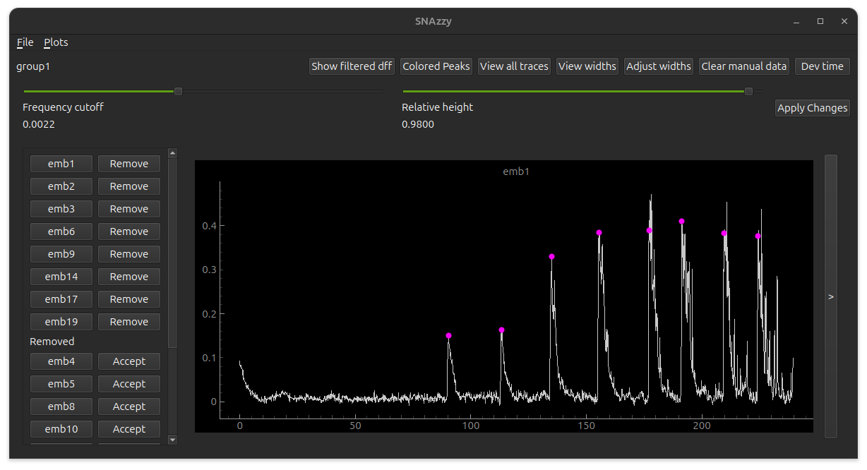
The description here refers to the image on the top of the file.
The top bar has buttons to change the data presentation. Below the top bar there are two sliders. The first is for the frequency cutoff, which controls how much the signal is smoothed for the finding peaks algorithm. The second is the peak width parameter, used to determine the start and end times of each peak. The sidebar presents which embryos are currently considered for plots and analysis, and which ones should be removed. You can toggle the embryo status between these two categories. In the main view you will see the DFF trace of the currently selected embryo. The pink dots represent the peak indices.
You can also visualize the signal from each channel, by clicking on the button with a > in the right of the screen.
This window will present the signal from each channel and also the hatching point, which can be changed manually by dragging the line if needed.
Manually changing peak data#
By pressing shift + left mouse click you can add a new peak to the plot.
Because we usually have many points over the X axis, it can be hard to click exactly where we want the peak index to land.
To help with this, the actual peak index after clicking in the local maximum value for a small window around the point that was clicked.
By pressing CTRL + left mouse click you can remove a peak.
It also works on a small X axis range just like when adding new peaks.
The peak width can also be adjusted. Click the button ‘Adjust widths’ to display handles on the peak boundaries. To change the width, just drag the line to the desired position.
The manual data is saved in peak_detection_params.json, in a key named embryos.
Click ‘Clear manual data’ to remove the manual data for the current sample of all samples at once.
View embryo movies#
If you haven’t removed the individual movies that were cropped from raw data, you can visualize them in the GUI.
Note
When running the pipeline, set the variable clean_up_data = False to keep the cropped movies.
The embryos must be placed inside the dataset directory, in a directory named embs.
If there are no files available to show, the GUI will simply display an error message.
If there are files, you can select one and see the movie in sync with the DFF trace.